Intro to R/RStudio

Author

StatMind

Published

January 7, 2024

1 Intro

1.1 Download and Install R

To download and install R, go to r-project website, and then choose a mirror, e.g., your country of residence or a nearby country. For Africa, you could pick South Africa but probably any country will do. Make sure to download the right version (Mac or Windows), and follow the instructions on your screen.

Tip

For those of you who use a laptop provided by your organization, you might need administrator rights to install new software. In those cases, you have to contact the IT-person!

1.2 Download and Install RStudio

R works fine without RStudio. However, RStudio - which is a so-called Integrated Development Environment or IDE - makes working with R much easier.

Even though you will see R, and the R logo, on your computer, we recommend downloading and installing RStudio, after downloading and installing R. Once RStudio is installed, you can forget about R. Opening RStudio automatically picks up the version of R installed on your computer.

To download and install RStudio, go to the posit.co website, and select the latest version for your platform (Windows or Mac). The site gives you the option to download R as the first step, but we already did that, so you can skip that step!

1.3 Opening RStudio

Once R and RStudio have been installed successfully, you can open RStudio (preferably by clicking on the RStudio logo on your desktop or task bar). The opening screen should look like this:

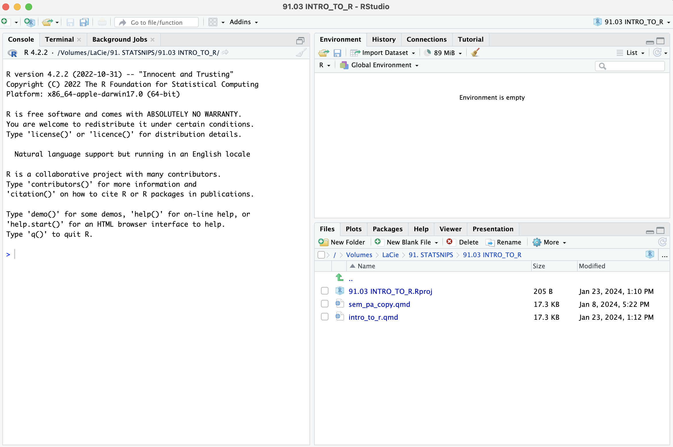
Initially, the screen is divided in three parts.
1. On the left, you see the console. In the console, you can type commands. The console will also display the output of the commands you give R.
2. On the top right, there is a panel with four tabs, including a tab labeled Environment. The environment is currently empty.
3. On the bottom right, there is a panel which shows you the files in a directory (e.g., your working directory). Another tab shows you any plots or figures you produce using R. Yet another tab gives information on the packages currently installed on your computer. Clicking on any of these packages produces the vignettes of these packages, including the functions of these packages and how to use them.

For now, just let the information sink in. Nevertheless, it helps to browse through all the tabs in the panels on the right. Most likely, you will a lot of the information not very helpful, yet, but over time you will become familiar with the contents. Just do not worry: knowing the very basics of R can get you very far!

1.4 Some Things You Need to Know

1.4.1 Base R and Packages

With the installation of R, you have access to Base R, and a couple of popular packages. And really, Base R has a lot to offer.

However, what makes R so popular, is the enormous number of packages developed by the community of R-users. At the time of writing (early 2024), there are over 20 thousand packages that you can install and use, free of charge. In 2021, R reported 17 thousand packages, and in 2023 19 thousand. The current growth rate is around one thousand per year.

It goes without saying that it is impossible for anyone to keep track of all existing and new packages. Luckily, there is no need to do so. Because of the large community of users of R, you can find a suitable package for your needs via Google.

For most of (y)our statistical tasks, there are a number of popular packages that we recommend and will make use of. But then again, with experience over time you will develop your own preferences and start using packages that we don’t know.

1.4.2 Installing and Using Packages

The vast majority of the over 20 thousand packages are not part of Base R. Some packages (e.g., stats, foreign) are installed with the installation of R.

For example, one of the packages we often use, is readstata13. The package has a function read.dta13() that reads data files produced in a commercial statistical software program called STATA. In order to install this package, we can either use the Install button under the Packages tab in the bottom right panel, or - our preferred way of working - use the install.packages() command.

We can type in the command in the console, or as a line of code in a script. If we include it in a script, then we have to be aware of the fact that the package will be installed every time we (re)run the script, which is not necessary. If, we use it in a script, then we make the command line a comment line, by adding “#” at the beginning. R ignores the comment lines (and everything that follows a “#”). In the script below, the line is just a reminder that we have installed the package. Many R-users, for good reason, prefer to install packages from the console rather than in a script.

Once the package (here, readstata13) has been installed, we do not have access yet to the functions in the package. We first have to invoke them via the library() command. This has to be done in every new session!

# install.packages("readstata13")
library(readstata13)

So, it’s good to remember:
1. Installing packages has to be done only once (per device).
2. Invoking the functions of a package has to be done in every session!

The first rule is not entirely true. R is regularly updated, in major and minor revisions. At present, the major version of R is 4, and the minor one is 2.2. This information is shown when starting a new session, and can be retrieved using R.version. If you install a newer version of R, then all packages that you have installed, are gone, and have to be installed again!

R.version

               _                           
platform       x86_64-apple-darwin17.0     
arch           x86_64                      
os             darwin17.0                  
system         x86_64, darwin17.0          
status                                     
major          4                           
minor          2.2                         
year           2022                        
month          10                          
day            31                          
svn rev        83211                       
language       R                           
version.string R version 4.2.2 (2022-10-31)
nickname       Innocent and Trusting

1.4.3 When to Update R

That leaves the question, should I update R, and if yes, how often?

Packages developed under a version of R, are backwards compatible. That is, if you have installed the latest version of R (4.2.3, at the time of writing), then all packages developed under older version of R should work. Using packages developed under a recent version of R, may cause problems when using an older version of R.

As a kind of routine, I install new versions of R every three to six months, or whenever I get warning messages that a package I want to use, was built under a newer version of R.

1.5 Pros and Cons of R

We use R because of the following benefits:

It is free.
It is extremely powerful.
It can do almost anything you can dream (or have nightmares) of.
The large user community makes it fairly to find examples that you can adapt.

However, compared to other software, there are some drawbacks.

Not everyone likes coding.
The learning curve is steep, implying that as a beginner you spend a lot of time on figuring out why your code doesn’t work.

One of our aims in this introduction is to overcome these drawbacks. In most cases, we do not spend a lot of time on coding. We pick examples from Internet sources, and we adapt the code to our situation (our data).

1.6 Useful Sources

For 99% of the basics (reading data; manipulating data; descriptive and inferential statistics; graphs), you can make use of examples on helpful websites.

We would recommend:

Quick-R, and
Cookbook for R.

2 Let’s Start!

2.1 R/RStudio as a Calculator

You can use R as a simple calculator.

You can make calculations in R, either from the console or from a script.

2+3     # Addition

[1] 5

10-6    # Subtraction

[1] 4

5*4     # Multiplication

[1] 20

20/4    # Division

[1] 5

3^2     # Exponentiation

[1] 9

sqrt(9) # Square Root

[1] 3

9^(1/2) # Square Root

[1] 3

2.2 Objects

Using R as a calculator, interactively, as above has the disadvantage that the result is lost. If you want to keep the results for later calculations, then it is preferable to store the results.

In R, results are stored as objects. For example, if we want to compute the future value (fv) of our present savings (pv) after n years, given an interest rate of i percent, we can use the following commands.

pv <- 10000  # present value of savings
i  <- 5/100  # interest rate (5%)
n  <- 3      # number of years ahead
fv <- pv*((1+i)^n)
fv <- format(round(as.numeric(fv), 0), nsmall=0, big.mark=",")
cat("The future value of our savings is", fv)

The future value of our savings is 11,576

We can conclude that the future value of our savings will be € 11,576, in 3 years from now.

Note

Note that we have used a couple of tricks in the code, to show the result in a nice manner (no decimals, or euro cents; and a comma to separate the thousands).

2.3 Script

Even in the relatively simple computation above, you see that it is easily looks complex. Especially the command for showing the output in a reader-friendly manner, took us some time Googling the best way to do it. Once we know how to do it, we don’t want to Google it again next time - or in similar computations.

For that reason, it is better to save all your useful commands in a script. Rather than keying everything in the console, we can combine all the commands in a script, and then run the script.

To open a script, just use File > New File > R-script. Alternatively, you can open other types of files (Notebooks; Markdowns; Quarto Files), that allow you to add annotations, and make your file readable, even to others.

Note

Actually, the document you are reading right now, is a Quarto file, with both text and R-code. The additional advantage of Quarto documents is that you can publish them, and share it with others.

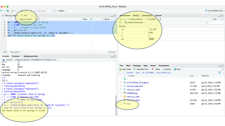
In the picture below, you see that:

We have copied the commands to a script (fv.R).
We have run the script, and the output appears in the console.
The environment tab displays all the objects that we have created.
In the files tab, the script (fv.R) is visible. The script is open, but if it’s open you can open it by clicking it.

2.4 Reading Data

There are many ways to read your data into R. For small data sets, you can easily do it within R.

For larger data sets, and/or the data sets that you have obtained from others, the most common way of sharing data is in text or Excel files.

2.4.1 Manual Data Entry

For the sake of the example, we will show you how to create data sets within R. It helps you understand how R is organized.

Suppose that we have a data on 5 students. We have recorded their scores on two parts of an exam. The total score on the exam is the sum of the two parts (maximum 100). We also recorded the names and gender of the students.

Name	Grade1	Grade2	Gender
Anna	20	25	F
Ben	30	20	M
Charles	40	50	M
Don	30	40	M
Eve	25	40	F

In R, a data frame is a set of vectors (columns). Here, we have 4 vectors (or columns, or variables), each of length 5.

We first define the 4 vectors, as combinations of 5 values each. We do so with the c() function. This function is widely used for combining elements, and the c makes it easy to remember (even though the c is derived from concatenation rather from combination!).

Once we have defined the four vectors, we combine them in a data frame using the data.frame() command.

name   <- c("Anna","Ben","Charles","Don","Eve")
grade1 <- c(20,30,40,30,25)
grade2 <- c(25,20,50,40,40)
gender <- c("F","M","M","M","F")
students <- data.frame(name,grade1,grade2,gender)
students

2.4.2 Read Data from Files

For larger data sets, entering data in R as we did above, is inconvenient, and error-prone.

It is better to organize your data in, for example, Excel. Many providers offer data in so-called csv-format. csv stands for comma separated values. This format is a text-file, with data organized in rows (observations; cases; or records), and the variables in columns. The first line often contains the labels of the columns, or headers. Before you start reading the data, make sure that you know whether a header line is included or not!

The csv-file can be read from your local computer, but sometimes the data are stored on a (public) url.

In our example, we have stored the csv-file with the information on students on GitHub. We can read the file directly, without downloading. By default, the read.csv() function assumes that the data file includes a header line, so it’s not necessary to add a header=TRUE argument. We store the information in a new object(s2).

s2 <- read.csv(url("https://raw.githubusercontent.com/statmind/statsnips/main/students_csv.csv"))
s2

2.4.3 Manipulating Data

Once the raw data have been read, we can start working with it. It is common to edit and manipulate the data before analysis.

For example, some grade scores may contain errors (e.g., grade1 is higher than the maximum of 50, or missing). In those cases, you might have to go back to the source, or if that’s not an option, correct or leave out the data. In our example, the data contains no obvious errors (which is different from stating that the data is correct!).
Data manipulation is needed if we are interested in analyzing the total score on the exam, which is just the sum of grade1 and grade2. We can create new variables, recode existing variables, and so on.

It is important to know that variables (or columns) in a data frame are referred to by dataframe$column. The variable grade1, in data frame s2 for example, can be accessed by s2$grade1.

s2$exam <- s2$grade1 + s2$grade2
s2

2.5 Workflow

Working with R and RStudio is easiest when using the following steps:

Create a folder on your computer, for your data project.
Open RStudio, and create a new project (File > New Project), using the existing folder created in step 1.
Automatically, files will be read and written in this project folder, and you do not have to use the full and lengthy path names.
Open a (new) script, and use comments (lines), because tomorrow you may have forgotten the logic of the code you wrote today!
It is absolutely essential to safeguard (i) the raw data, and the (ii) latest version of your script. Running the latest script on the raw data should reproduce everything you have done. So, make regular backups of these files!!

flowchart LR
  A[New Project] --> B{Raw Data}
  B --> C(Backup!)
  B --> D{Script}
  D --> E[Read Data]
  D --> F[Manipulate]
  D --> G[Analyze]
  D --> H(Backup!)

3 Practice

It helps to use our sample data sets, to try new things.

Looking at the small data set of 5 students, we can ask many questions:

How many students are male?
What is the average score on grade1 and grade2?
Is there a relationship between the scores on the two parts of the exam?
How long are the names of our students?
And so on …

As an example, let’s look at the second and third question.

In Quick-R, we can find several options to get descriptive statistics.

One way is the sapply() function, with the argument mean (avarage).

# From Quick-R: get means for variables in a data frame
# Excluding missing values
sapply(s2, mean, na.rm=TRUE)

Warning in mean.default(X[[i]], ...): argument is not numeric or logical:
returning NA

Warning in mean.default(X[[i]], ...): argument is not numeric or logical:
returning NA

  name grade1 grade2 gender   exam 
    NA     29     35     NA     64

This results in a warning, since our data set contains non-numeric data (characters, in name and gender) which cannot be averaged.

Note

Does it surprise you that the mean on **exam** is 64? Why (not)?

We can select the relevant columns (2 and 3). In the expression s2[rows,columns], we select rows and columns between the brackets [rows,columns]. Before the comma, we specify all rows by leaving it blank; after the comma, we specify columns 2 to 3.

sapply(s2[,2:3], mean, na.rm=TRUE)

grade1 grade2 
    29     35

For the relationship between grade1 and grade2, it would be nice to display it graphically. We can do so in a scatter plot. We can again consult Quick-R, and find some examples.

We copy and paste the code for a simple scatterplot, and adapt it to our data.

# Simple Scatterplot
attach(s2)

The following objects are masked _by_ .GlobalEnv:

    gender, grade1, grade2, name

plot(grade1, grade2, main="Scatterplot of Grades",
   xlab="Grade 1", ylab="Grade 2", pch=19)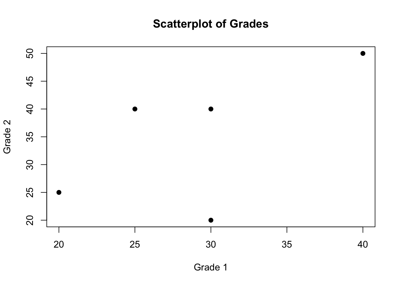

Tip

The attach(s2) command tells R to find the variables in the commands that follow, in the s2 data frame. Without the attach() command, we would have to specify s2$grade1 and s2$grade2 in the plot() command. In general, it is considered bad practice to use the attach() command, since it is prone to errors (especially if you forget to use detach() if you switch to another data frame).

4 Summary

In this StatSnip, we have introduced R and Rstudio.

Main points to take-away:

Familiarize yourself with the 4 panels in RStudio!
Know how to install packages, and how to invoke the functions in these packages!
Practice using R as a calculator.
Create objects using the “<-” operator. Check if these objects pop up in the Environment tab.
Follow the workflow. Start by creating a project folder for your data project (even for learning R), and open an R-project.
Practice entering data in R, and create data frames.
Try to read (csv) files that you have created via Excel.
Open a script. Type in commands in the script, and run specific lines (by highlighting) in the script, or the whole script.
Use Google to figure out how to do things in R that we have not (yet) discussed.
Browse through the examples in Quick-R and Cookbook-for-R!
Play with the sample data, and try new things!