Path models consist of independent and dependent variables depicted graphically by rectangles.
Variables that are independent variables, and not dependent variables, are called exogenous.
Graphically, exogenous variables have only arrows pointing to (endogenous) variables. No arrows point at exogenous variables.
Endogenous variables are:
Strictly dependent variables, or
Both independent and dependent.
Graphically, endogenous variables have at least one arrow pointing at them.
We will use an example from the field of high-performance organizations (HPOs). De Waal has developed an HPO model in which organizational performance is indicated by five factors:
Continuous Innovation (CI)
Openness & Action Orientation (OAO)
Management Quality (MQ)
Employee Quality (QEMP)
Long-Term Orientation (LTO).
For illustrating path analysis, we will use a sample data set with three of the five factors (MQ, QEMP, and OAO). For 250 organizations, we have data on the three indicators, and on two aspects of performance, namely financial performance (FPF) and non-financial performance (NFPF). All variables are measured on a five point scale.
Note
Actually, all measures - including the three HPO factors - are composite measures (not directly observed latent variables), based on observed answers to a set of questions (items). In another StatSnip we will discuss the ways to include latent variables.
Our model, or path diagram, is:
With regression analysis, we can estimate models with one dependent variable. Of course, for the model above we can run two separate regression models, but that would not be the same (e.g., we wouldn’t know if and how the dependent variables are related). The challenge of using regression analysis would become bigger, if we would include mediating variables (like an effect of MQ on OAO).
In this StatSnip, we will:
Show you how regression analysis is just a special case of a more general path analysis.
Show you how to perform path analysis in STATA.
Show you how to achieve the same results in the free R-software, using the lavaan package.
Discuss model comparisons, model improvements, and the use of goodness-of-fit statistics.
2 Regression Analysis and Path Analysis
Regression analysis estimates the relationship between one dependent and one or more independent variables. Path analysis is an extension of regression models, and can include more than one endogenous variable and mediating variables that are both explained in the model (by other exogenous or endogenous variables) and explain other (endogenous) variables.
Even though a path analysis with one endogenous variable, and, say, three exogenous variables is equivalent to a regression model with one dependent and three independent variables, the commands and functions use terms and layouts of the results that make users feel uncomfortable.
So, what we will do first, is to estimate the model below, using regression analysis and path analysis, in STATA and in R.
      mqr            qempr            oaor            fpfr          nfpfr
 Min.   :1.000   Min.   :1.000   Min.   :1.000   Min.   :1.00   Min.   :1.000
 1st Qu.:2.000   1st Qu.:2.000   1st Qu.:2.000   1st Qu.:3.00   1st Qu.:3.000
 Median :3.000   Median :3.000   Median :3.000   Median :3.00   Median :4.000
 Mean   :3.064   Mean   :2.976   Mean   :3.132   Mean   :3.26   Mean   :3.404
 3rd Qu.:4.000   3rd Qu.:4.000   3rd Qu.:4.000   3rd Qu.:4.00   3rd Qu.:4.000
 Max.   :5.000   Max.   :5.000   Max.   :5.000   Max.   :5.00   Max.   :5.000
The data set contains the responses from 250 respondents, on the five variables. All variables end with r (e.g., management quality mq becomes mqr), to indicate that all variables have been recoded from into a 5-point scale (1=very poor, 5=very good), for sake of ease. Above, we have added summary information on the five variables, and the correlations between the variables.
2.2 The Model
We want to estimate a regression model with one dependent variable (fpfr) and three independent variables (mqr, qempr, and oaor).
We use the sembuilder in STATA to draw the diagram.
The nice thing about the sembuilder is that the model can be built graphically, and estimated directly. Behind the scenes, STATA builds the command which then can be adapted if needed.
Tip
It is often faster to use commands rather than the Graphical Unit Interface (sembuilder). With more complex models, it takes several steps to come to the final model, and making the changes in the diagram consumes more time. It is best to make the base model and the final model using the GUI, and everything in between in commands (preferably in a STATA DO-file).
If indeed the two approaches are identical, then (among others):
The paths in SEM should be the same as the regression coefficients in regression analysis
The explained variance (coefficient of determination \[R^{2}\]) should be the same.
Well, everything is the same. But since - in both STATA and R - the output stemming from both approaches are way different, it is a bit of a challenge to reach that conclusion.
2.2.1 STATA
Regression in STATA produces the type of output that you may be familiar with:
The (standardized) regression coefficients coefficients are in the circle marked green. The \[R^{2}\] is in the bluish oval.
The (standardized) regression coefficients are the same as the paths in the diagram below. Again, we have emphasized them in green. The equivalent of the coefficient of determination in regression analysis, is 1 minus the (unexplained) variance in the diagram: \[1 - .57=.43\].
The output of SEM entails more than what is depicted in the diagram. It is possible to display a lot of it in the diagram, but it easily gets crowded, and the main aim of the diagram is to focus the attention of your audience on the key aspects of the analysis.
Detailed output is shown below.
2.2.2 R (lavaan)
The advantages of STATA for using SEM are (i) the excellent documentation, and the (ii) the GUI (sembuilder). The disadvantage of commercial software like STATA and SPSS is that it doesn’t come cheap.
The lavaan package of R offers a great free-of-cost alternative. There is to the best of our knowledge no GUI available (yet), but this is minor drawback. In most cases, we use sembuilder for the final model only - and R does offer additional packages to achieve more or less the same.
Below, we have used the lavaan package, to estimate the regression model as a path analysis. A description of the package and a user-friendly tutorial with examples can be found here.
Let’s start by running a regression model, using the lm() function of R. In order to get the standardized regression coefficients, we install the lm.beta package. The function lm.beta() applied to the model that is fit with lm(), prodices the standardized regression coefficients.
lavaan 0.6.17 ended normally after 1 iteration

  Estimator                                         ML
  Optimization method                           NLMINB
  Number of model parameters                         4

  Number of observations                           250

Model Test User Model:

  Test statistic                                 0.000
  Degrees of freedom                                 0

Parameter Estimates:

  Standard errors                             Standard
  Information                                 Expected
  Information saturated (h1) model          Structured

Regressions:
                   Estimate  Std.Err  z-value  P(>|z|)   Std.lv  Std.all
  fpfr ~
    mqr               0.187    0.038    4.861    0.000    0.187    0.308
    qempr             0.288    0.034    8.450    0.000    0.288    0.421
    oaor              0.105    0.055    1.910    0.056    0.105    0.119

Variances:
                   Estimate  Std.Err  z-value  P(>|z|)   Std.lv  Std.all
   .fpfr              0.435    0.039   11.180    0.000    0.435    0.567
You will find that R gives the same results as STATA.
In lavaan, you work in two steps.
In step 1, you formulate the complete model. For a simple regression model, we only have to specify the regression model which is identical to what you feed into the lm() function: fpfr ~ mqr + qempr + oaor.
In the second step, you use lavaan’s CFA() function to estimate the model defined in step 1.
The standardized coefficients (paths), appear in the column Std.all.
2.3 A Path Model With Two Endogenous Variables
Hopefully, you will now feel confident that (whether you ar using STATA or R), regression analysis is just a very special case of path analysis.
Path analysis enables you to estimate models which are more complex, and also more realistic, than a regression model with one independent variable.
For example, let’s have a look at the model we showed at the beginning, in which we have added non-financial performance (nfpfr) as a second dependent variable. There’s nothing wrong with the term dependent variable, but for consistency, it is better to speak of endogenous variables.
Below, we show the diagram produced by STATA.
If you don’t have STATA at your disposal, then we can use lavaan to get the same results. Note that we have explicitly added covariances (“~~”) between the exogenous in the model. This does not affect the results, since covariances are assumed. Adding them to the model sees to it that they are displayed in the output.
The regressions part shows the paths (regression coefficients). The standardized coefficients are in the Std.all column. The first block contains the coefficients for the endogenous variable fpfr, and the second block for nfpfr. They are identical (in to decimals precision) to paths in the figure above.
The standardized covariances (correlations, that is), between the exogenous variables mqr, qempr, and oaor are the same as the numbers at the two-headed arrows on the left of the figure.
We have specified a covariance (or correlation, since we use standardized results) between the error terms of the two endogenous variables. This correlation is close to zero (.03), and not significantly different from zero. We might leave it out of the model, by constraining it to zero.
The variances of interest are those of the error terms of the endogenous variables. The variance of the error term of fpfr (.fpfr, in the output) is .567, and hence the explained variance is 1 - .567 = .433. The variance of nfpfr explained by the model is 1 - .728 = .272.
A part of the output that we have not discussed yet, is the test statistic, and the degrees of freedom. What essentially happens is that the model estimates the model parameters, given the matrix of variances and covariances in the data. In a saturated model, we have a system of equations with as many unknowns as we have parameters - and the model fits the data perfectly.
2.4 Non-Saturated Models
We can simplify the model, by leaving out some of the paths, and/or covariances. Leaving out the paths, is synonymous to constraining them to zero. By doing so, we have more degrees of freedom in fitting the model. At the same time, our model may not fit the data, e.g., if a left out path is in fact significantly different from zero.
The logic of your model should follow theory. If literature has found, or if you hypothesize, that mqr has no bearing on non-financial performance, and oaor has no effect on financial performance, and in addition financial and non-financial performance are uncorrelated, given the exogenous variables, you can estimate and test the following model:
Since we have left out two paths, and constrained covariance between the error terms of the endogenous variables to zero, we have gained three degrees of freedom. This allows us to test our model.
The test uses a chi-square statistic, based on the differences between the matrix of variances and covariances of the variables in the analysis, and the implied matrix based on the parameter estimates. Ideally, our model replicates the data perfectly, and the chi-square is close to zero. Here, our chi-square is significantly different from zero, and, hence, the model does not fit the data very well.
Tip
There has been a longstanding discussion on the best set of statistics for evaluating the model fit. The outcome of that discussion is that it wise to look at a couple of statistics. For an overview, see the article by Hoopen et al (2008). The bottom line is that the researcher should use and report:
The chi-square statistic with its degrees of freedom, and the p-value.
The Root Mean Square Error of Approximation (RMSEA) should be smaller than .07.
The Standard Root Mean Square Residual (SRMR) is ideally lower than .05 but values up to .08 are considered acceptable.
Comparative Fit Index (CFI), should be higher than .95 (although some use .90).
These measures can be obtained in lavaan.
Below, we estimate the model in R, with lavaan. Note that in the code, we can just leave out the paths that we assume to be zero. Constraining the covariance between the error terms of the endogenous variables, is specified by multiplying the right hand side of the covariance (“~~”) to zero.
lavaan 0.6.17 ended normally after 26 iterations

  Estimator                                         ML
  Optimization method                           NLMINB
  Number of model parameters                        12

  Number of observations                           250

Model Test User Model:

  Test statistic                                19.521
  Degrees of freedom                                 3
  P-value (Chi-square)                           0.000

Model Test Baseline Model:

  Test statistic                               379.632
  Degrees of freedom                                10
  P-value                                        0.000

User Model versus Baseline Model:

  Comparative Fit Index (CFI)                    0.955
  Tucker-Lewis Index (TLI)                       0.851

Loglikelihood and Information Criteria:

  Loglikelihood user model (H0)              -1724.379
  Loglikelihood unrestricted model (H1)      -1714.618

  Akaike (AIC)                                3472.758
  Bayesian (BIC)                              3515.016
  Sample-size adjusted Bayesian (SABIC)       3476.975

Root Mean Square Error of Approximation:

  RMSEA                                          0.148
  90 Percent confidence interval - lower         0.090
  90 Percent confidence interval - upper         0.214
  P-value H_0: RMSEA <= 0.050                    0.004
  P-value H_0: RMSEA >= 0.080                    0.972

Standardized Root Mean Square Residual:

  SRMR                                           0.052

Parameter Estimates:

  Standard errors                             Standard
  Information                                 Expected
  Information saturated (h1) model          Structured

Regressions:
                   Estimate  Std.Err  z-value  P(>|z|)
  fpfr ~
    mqr               0.232    0.030    7.657    0.000
    qempr             0.292    0.034    8.538    0.000
  nfpfr ~
    qempr             0.222    0.046    4.790    0.000
    oaor              0.341    0.060    5.710    0.000

Covariances:
                   Estimate  Std.Err  z-value  P(>|z|)
  mqr ~~
    qempr             0.538    0.122    4.398    0.000
    oaor              0.932    0.109    8.578    0.000
  qempr ~~
    oaor              0.303    0.083    3.644    0.000
 .fpfr ~~
   .nfpfr             0.000

Variances:
                   Estimate  Std.Err  z-value  P(>|z|)
   .fpfr              0.442    0.040   11.180    0.000
   .nfpfr             0.838    0.075   11.180    0.000
    mqr               2.092    0.187   11.180    0.000
    qempr             1.647    0.147   11.180    0.000
    oaor              0.995    0.089   11.180    0.000
Code
summary(fit4, standardized =TRUE)
lavaan 0.6.17 ended normally after 26 iterations

  Estimator                                         ML
  Optimization method                           NLMINB
  Number of model parameters                        12

  Number of observations                           250

Model Test User Model:

  Test statistic                                19.521
  Degrees of freedom                                 3
  P-value (Chi-square)                           0.000

Parameter Estimates:

  Standard errors                             Standard
  Information                                 Expected
  Information saturated (h1) model          Structured

Regressions:
                   Estimate  Std.Err  z-value  P(>|z|)   Std.lv  Std.all
  fpfr ~
    mqr               0.232    0.030    7.657    0.000    0.232    0.384
    qempr             0.292    0.034    8.538    0.000    0.292    0.428
  nfpfr ~
    qempr             0.222    0.046    4.790    0.000    0.222    0.274
    oaor              0.341    0.060    5.710    0.000    0.341    0.327

Covariances:
                   Estimate  Std.Err  z-value  P(>|z|)   Std.lv  Std.all
  mqr ~~
    qempr             0.538    0.122    4.398    0.000    0.538    0.290
    oaor              0.932    0.109    8.578    0.000    0.932    0.646
  qempr ~~
    oaor              0.303    0.083    3.644    0.000    0.303    0.237
 .fpfr ~~
   .nfpfr             0.000                               0.000    0.000

Variances:
                   Estimate  Std.Err  z-value  P(>|z|)   Std.lv  Std.all
   .fpfr              0.442    0.040   11.180    0.000    0.442    0.575
   .nfpfr             0.838    0.075   11.180    0.000    0.838    0.775
    mqr               2.092    0.187   11.180    0.000    2.092    1.000
    qempr             1.647    0.147   11.180    0.000    1.647    1.000
    oaor              0.995    0.089   11.180    0.000    0.995    1.000
From the massive output, we conclude:
The effects of the exogenous variables are significantly different from zero.
All effects are moderate to strong, in the .3 to .4 order of magnitude.
The model fit is poor. The chi-square statistic is significantly different from zero. The RMSEA is .149, which is well above the upper limit of .07.
2.5 Model Improvement
If, like above, we have a model with a poor fit, we can try to improve it by adding loosening the constraints. In our model, we have constrained three parameters to zero, which explains the 3 degrees of freedom in the model.
One strategy to improve the model, is by computing what would happen to our chi-square statistic if we would do away with the constraint.
In SEM jargon, we use modification indices to determine the model improvement of of adding constrained parameters. A problem of listing modification indices, is that the software doesn’t think. For example, linking the endogenous variables can be done in various ways: by adding (back) the covariance that we constrained to zero; by adding a path from fpfr to nfpfr, or a path the other way round. All of these options have some impact. That is, they do improve the model. Whether the path or parameter makes sense, is a different matter.
Below, we use the modindices() function, to detect improvements that are substantial and make sense. We can store the output in an object, which is a data frame (with labeled variables). In order to narrow down the output, we can apply a filter. For example, in the code we only consider improvements that have either fpfr or nfpfr on the left hand side (variable lhs) in a regression (variable op == “~”).
Code
mi <-modindices(fit4, sort =TRUE, maximum.number =20)mi
Our selection contains 4 rules. The last two lines suggest paths from fpfr to nfpfr, or the other way round. A path from fpfr to nfpfr (we could adjust nfpfr ~ qemprr + oaor, into nfpfr ~ qempr + oaor + fpfr) would decrease chi-square by 2.4 (out of 19.5). By doing so, we would add an indirect effect of the exogenous variables mqr and qempr, via fpfr, on nfpfr. A more substantial improvement can be obtained by adding one of the two omitted paths: the path from mqr to nfpfr. The chi-square will go down from 19.5 to 19.5 minus 15.2.
lavaan 0.6.17 ended normally after 28 iterations

  Estimator                                         ML
  Optimization method                           NLMINB
  Number of model parameters                        13

  Number of observations                           250

Model Test User Model:

  Test statistic                                 3.849
  Degrees of freedom                                 2
  P-value (Chi-square)                           0.146

Model Test Baseline Model:

  Test statistic                               379.632
  Degrees of freedom                                10
  P-value                                        0.000

User Model versus Baseline Model:

  Comparative Fit Index (CFI)                    0.995
  Tucker-Lewis Index (TLI)                       0.975

Loglikelihood and Information Criteria:

  Loglikelihood user model (H0)              -1716.543
  Loglikelihood unrestricted model (H1)      -1714.618

  Akaike (AIC)                                3459.086
  Bayesian (BIC)                              3504.865
  Sample-size adjusted Bayesian (SABIC)       3463.654

Root Mean Square Error of Approximation:

  RMSEA                                          0.061
  90 Percent confidence interval - lower         0.000
  90 Percent confidence interval - upper         0.153
  P-value H_0: RMSEA <= 0.050                    0.316
  P-value H_0: RMSEA >= 0.080                    0.457

Standardized Root Mean Square Residual:

  SRMR                                           0.019

Parameter Estimates:

  Standard errors                             Standard
  Information                                 Expected
  Information saturated (h1) model          Structured

Regressions:
                   Estimate  Std.Err  z-value  P(>|z|)
  fpfr ~
    mqr               0.232    0.030    7.657    0.000
    qempr             0.292    0.034    8.538    0.000
  nfpfr ~
    mqr               0.208    0.052    4.022    0.000
    qempr             0.188    0.046    4.117    0.000
    oaor              0.157    0.074    2.123    0.034

Covariances:
                   Estimate  Std.Err  z-value  P(>|z|)
  mqr ~~
    qempr             0.538    0.122    4.398    0.000
    oaor              0.932    0.109    8.578    0.000
  qempr ~~
    oaor              0.303    0.083    3.644    0.000
 .fpfr ~~
   .nfpfr             0.000

Variances:
                   Estimate  Std.Err  z-value  P(>|z|)
   .fpfr              0.442    0.040   11.180    0.000
   .nfpfr             0.787    0.070   11.180    0.000
    mqr               2.092    0.187   11.180    0.000
    qempr             1.647    0.147   11.180    0.000
    oaor              0.995    0.089   11.180    0.000
By adding one parameter, the model’s chi-square goes down to 3.85 (not exactly 19.5 minus 15.2; the MI’s are approximations), with 2 degrees of freedom. The p-value is 0.146, which means that it’s not significantly different from zero. Our data matches the model implied variance-covariance matrix quite well.
The other goodness–of-fit statistics are also good. In our report we can say that:
The χ2 (df=2) = 3.85 (p=.15), indicating a good fit.
The RMSEA = 0.06, below the upper limit of .07. The probability (Pclose) of RMSEA being smaller than 0.05 is .32.
The SRMR = 0.02, which suggests a good fit.
The CFI is very close to 1.
Source Code
---title: "Structural Equation Analysis: Path Analysis"author: "StatMind"date: 2024/01/07format: html: df-print: paged code-fold: true code-tools: truenumber-sections: truetoc: truetoc-depth: 4toc-title: In this StatSnipeditor: visual---## IntroPath models consist of independent and dependent variables depicted graphically by rectangles.Variables that are independent variables, and not dependent variables, are called *exogenous*.Graphically, exogenous variables have only arrows pointing to (*endogenous*) variables. No arrows point at exogenous variables.Endogenous variables are:1. Strictly dependent variables, or2. Both independent and dependent.Graphically, endogenous variables have at least one arrow pointing at them.We will use an example from the field of *high-performance organizations (HPOs)*. [De Waal](https://www.mdpi.com/2071-1050/12/20/8507) has developed an HPO model in which organizational performance is indicated by five factors:1. Continuous Innovation (CI)2. Openness & Action Orientation (OAO)3. Management Quality (MQ)4. Employee Quality (QEMP)5. Long-Term Orientation (LTO).For illustrating path analysis, we will use a sample data set with three of the five factors (MQ, QEMP, and OAO). For 250 organizations, we have data on the three indicators, and on two aspects of performance, namely financial performance (FPF) and non-financial performance (NFPF). All variables are measured on a five point scale.::: callout-noteActually, all measures - including the three HPO factors - are composite measures (not directly observed latent variables), based on observed answers to a set of questions (items). In another StatSnip we will discuss the ways to include latent variables.:::Our model, or path diagram, is: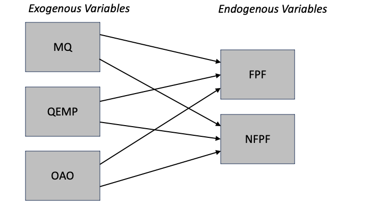With regression analysis, we can estimate models with one dependent variable. Of course, for the model above we can run two separate regression models, but that would not be the same (e.g., we wouldn't know if and how the dependent variables are related). The challenge of using regression analysis would become bigger, if we would include mediating variables (like an effect of MQ on OAO).In this StatSnip, we will:1. Show you how regression analysis is just a special case of a more general path analysis.2. Show you how to perform path analysis in STATA.3. Show you how to achieve the same results in the free R-software, using the *lavaan* package.4. Discuss model comparisons, model improvements, and the use of goodness-of-fit statistics.## Regression Analysis and Path AnalysisRegression analysis estimates the relationship between one dependent and one or more independent variables. Path analysis is an extension of regression models, and can include more than one endogenous variable and mediating variables that are both explained in the model (by other exogenous or endogenous variables) and explain other (endogenous) variables.Even though a path analysis with one endogenous variable, and, say, three exogenous variables is equivalent to a regression model with one dependent and three independent variables, the commands and functions use terms and layouts of the results that make users feel uncomfortable.So, what we will do first, is to estimate the model below, using regression analysis and path analysis, in STATA and in R.### The DataLet us first read the data.```{r}library(readstata13)hpo250 <-read.dta13("hpo250.dta")hpo250cormat <-cor(hpo250) # Correlation matrix of the 5 variablesround(cormat, 2) # Print, in 2 decimals summary(hpo250) # Key descriptives ```The data set contains the responses from 250 respondents, on the five variables. All variables end with *r* (e.g., management quality **mq** becomes **mqr**), to indicate that all variables have been recoded from into a 5-point scale (1=very poor, 5=very good), for sake of ease. Above, we have added summary information on the five variables, and the correlations between the variables.### The ModelWe want to estimate a regression model with one dependent variable (**fpfr**) and three independent variables (**mqr**, **qempr**, and **oaor**).We use the *sembuilder* in STATA to draw the diagram.The regression model is:$$fpfr = \beta_{0} + \beta_{1}*mqr + \beta_2*qempr + \beta_{3}*oaor$$The nice thing about the *sembuilder* is that the model can be built graphically, and estimated directly. Behind the scenes, STATA builds the command which then can be adapted if needed.::: callout-tipIt is often faster to use commands rather than the Graphical Unit Interface (*sembuilder*). With more complex models, it takes several steps to come to the final model, and making the changes in the diagram consumes more time. It is best to make the base model and the final model using the GUI, and everything in between in commands (preferably in a STATA DO-file).:::If indeed the two approaches are identical, then (among others):- The paths in SEM should be the same as the regression coefficients in regression analysis- The explained variance (coefficient of determination $$R^{2}$$) should be the same.Well, everything is the same. But since - in both STATA and R - the output stemming from both approaches are way different, it is a bit of a challenge to reach that conclusion.#### STATARegression in STATA produces the type of output that you may be familiar with: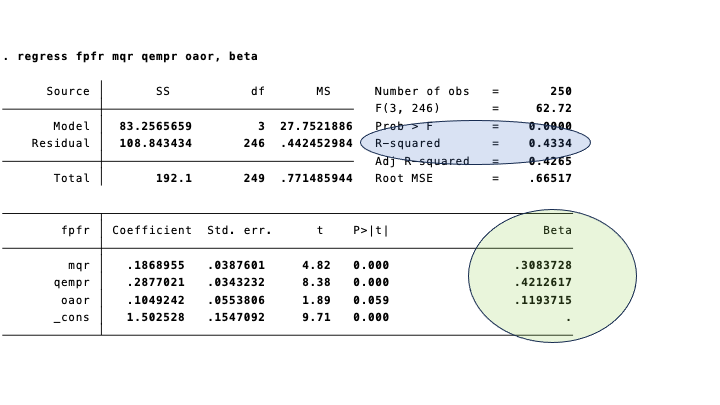The (standardized) regression coefficients coefficients are in the circle marked green. The $$R^{2}$$ is in the bluish oval.The (standardized) regression coefficients are the same as the paths in the diagram below. Again, we have emphasized them in green. The equivalent of the coefficient of determination in regression analysis, is 1 minus the (unexplained) variance in the diagram: $$1 - .57=.43$$.The output of SEM entails more than what is depicted in the diagram. It is possible to display a lot of it in the diagram, but it easily gets crowded, and the main aim of the diagram is to focus the attention of your audience on the key aspects of the analysis.Detailed output is shown below.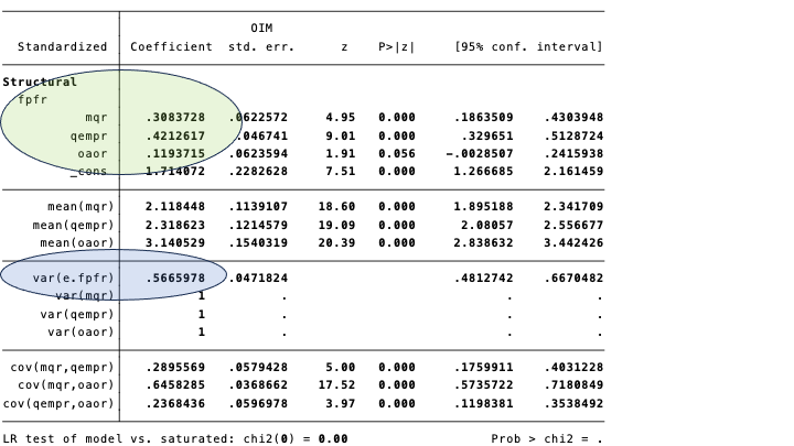#### R (lavaan)The advantages of STATA for using SEM are (i) the excellent documentation, and the (ii) the GUI (*sembuilder*). The disadvantage of commercial software like STATA and SPSS is that it doesn't come cheap.The *lavaan* package of R offers a great free-of-cost alternative. There is to the best of our knowledge no GUI available (yet), but this is minor drawback. In most cases, we use *sembuilder* for the final model only - and R does offer additional packages to achieve more or less the same.Below, we have used the *lavaan* package, to estimate the regression model as a path analysis. A description of the package and a user-friendly tutorial with examples can be found [here](https://lavaan.ugent.be/).Let's start by running a regression model, using the *lm()* function of R. In order to get the standardized regression coefficients, we install the *lm.beta* package. The function *lm.beta()* applied to the model that is fit with *lm()*, prodices the standardized regression coefficients.```{r}# Regression (lm())fitreg <-lm(fpfr ~ mqr + qempr + oaor,data=hpo250)summary(fitreg)library(lm.beta) # To obtain the standardized regression coefficientslm.beta(fitreg)```Let's now turn to *lavaan*. Don't forget to install the *lavaan* package before using it!```{r}# Regression (lavaan)# install.packages("lavaan", dependencies = TRUE)library(lavaan)model_reg2 <-'# regression fpfr ~ mqr + qempr + oaor 'fit2 <-cfa(model_reg2, data=hpo250)summary(fit2, standardized =TRUE)```You will find that R gives the same results as STATA.In *lavaan*, you work in two steps.1. In step 1, you formulate the complete model. For a simple regression model, we only have to specify the regression model which is identical to what you feed into the *lm()* function: *fpfr \~ mqr + qempr + oaor*.2. In the second step, you use *lavaan*'s *CFA()* function to estimate the model defined in step 1.The standardized coefficients (paths), appear in the column *Std.all*.### A Path Model With Two Endogenous VariablesHopefully, you will now feel confident that (whether you ar using STATA or R), regression analysis is just a very special case of path analysis.Path analysis enables you to estimate models which are more complex, and also more realistic, than a regression model with one independent variable.For example, let's have a look at the model we showed at the beginning, in which we have added non-financial performance (**nfpfr**) as a second dependent variable. There's nothing wrong with the term dependent variable, but for consistency, it is better to speak of endogenous variables.Below, we show the diagram produced by STATA.If you don't have STATA at your disposal, then we can use *lavaan* to get the same results. Note that we have explicitly added covariances ("\~\~") between the exogenous in the model. This does not affect the results, since covariances are assumed. Adding them to the model sees to it that they are displayed in the output.```{r}model_reg3 <-'# regression two dependent variables fpfr ~ mqr + qempr + oaor nfpfr ~ mqr + qempr + oaor # covariances mqr ~~ qempr mqr ~~ oaor qempr ~~ oaor 'fit3 <-cfa(model_reg3, data=hpo250)summary(fit3, standardized =TRUE)```Scrolling through the output:1. The *regressions* part shows the paths (regression coefficients). The standardized coefficients are in the *Std.all* column. The first block contains the coefficients for the endogenous variable **fpfr**, and the second block for **nfpfr**. They are identical (in to decimals precision) to paths in the figure above.2. The standardized covariances (correlations, that is), between the exogenous variables **mqr**, **qempr**, and **oaor** are the same as the numbers at the two-headed arrows on the left of the figure.3. We have specified a covariance (or correlation, since we use standardized results) between the error terms of the two endogenous variables. This correlation is close to zero (*.03*), and not significantly different from zero. We might leave it out of the model, by constraining it to zero.4. The variances of interest are those of the error terms of the endogenous variables. The variance of the error term of **fpfr** (**.fpfr**, in the output) is *.567*, and hence the explained variance is *1 - .567 = .433*. The variance of **nfpfr** explained by the model is *1 - .728 = .272*.A part of the output that we have not discussed yet, is the test statistic, and the degrees of freedom. What essentially happens is that the model estimates the model parameters, given the matrix of variances and covariances in the data. In a saturated model, we have a system of equations with as many unknowns as we have parameters - and the model fits the data perfectly.### Non-Saturated ModelsWe can simplify the model, by leaving out some of the paths, and/or covariances. Leaving out the paths, is synonymous to constraining them to zero. By doing so, we have more *degrees of freedom* in fitting the model. At the same time, our model may not fit the data, e.g., if a left out path is in fact significantly different from zero.The logic of your model should follow theory. If literature has found, or if you hypothesize, that **mqr** has no bearing on non-financial performance, and **oaor** has no effect on financial performance, and in addition financial and non-financial performance are uncorrelated, given the exogenous variables, you can estimate and test the following model: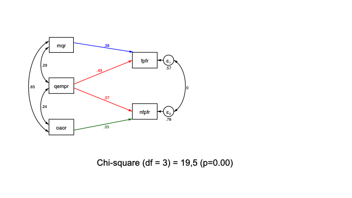Since we have left out two paths, and constrained covariance between the error terms of the endogenous variables to zero, we have gained three degrees of freedom. This allows us to test our model.The test uses a chi-square statistic, based on the differences between the matrix of variances and covariances of the variables in the analysis, and the *implied* matrix based on the parameter estimates. Ideally, our model replicates the data perfectly, and the chi-square is close to zero. Here, our chi-square is significantly different from zero, and, hence, the model does not fit the data very well.::: callout-tipThere has been a longstanding discussion on the best set of statistics for evaluating the model fit. The outcome of that discussion is that it wise to look at a couple of statistics. For an overview, see the article by [Hoopen et al (2008)](https://www.researchgate.net/publication/254742561_Structural_Equation_Modeling_Guidelines_for_Determining_Model_Fit). The bottom line is that the researcher should use and report:1. The chi-square statistic with its degrees of freedom, and the p-value.2. The Root Mean Square Error of Approximation (RMSEA) should be smaller than .07.3. The Standard Root Mean Square Residual (SRMR) is ideally lower than .05 but values up to .08 are considered acceptable.4. Comparative Fit Index (CFI), should be higher than .95 (although some use .90).These measures can be obtained in *lavaan*.:::Below, we estimate the model in R, with *lavaan*. Note that in the code, we can just leave out the paths that we assume to be zero. Constraining the covariance between the error terms of the endogenous variables, is specified by multiplying the right hand side of the covariance ("\~\~") to zero.```{r}model_reg4 <-'# regression two dependent variables fpfr ~ mqr + qempr nfpfr ~ qempr + oaor # variances and covariances mqr ~~ qempr mqr ~~ oaor qempr ~~ oaor # residual correlations fpfr ~~ 0*nfpfr 'fit4 <-cfa(model_reg4, data=hpo250)summary(fit4, fit.measures=TRUE)summary(fit4, standardized =TRUE)```From the massive output, we conclude:1. The effects of the exogenous variables are significantly different from zero.\2. All effects are moderate to strong, in the .3 to .4 order of magnitude.\3. The model fit is poor. The chi-square statistic is significantly different from zero. The RMSEA is .149, which is well above the upper limit of .07.### Model ImprovementIf, like above, we have a model with a poor fit, we can try to improve it by adding loosening the constraints. In our model, we have constrained three parameters to zero, which explains the 3 degrees of freedom in the model.One strategy to improve the model, is by computing what would happen to our chi-square statistic if we would do away with the constraint.In SEM jargon, we use *modification indices* to determine the model improvement of of adding constrained parameters. A problem of listing modification indices, is that the software doesn't think. For example, linking the endogenous variables can be done in various ways: by adding (back) the covariance that we constrained to zero; by adding a path from **fpfr** to **nfpfr**, or a path the other way round. All of these options have some impact. That is, they do improve the model. Whether the path or parameter makes sense, is a different matter.Below, we use the *modindices()* function, to detect improvements that are substantial and make sense. We can store the output in an object, which is a data frame (with labeled variables). In order to narrow down the output, we can apply a filter. For example, in the code we only consider improvements that have either **fpfr** or **nfpfr** on the left hand side (variable **lhs**) in a regression (variable **op** == "\~").```{r}mi <-modindices(fit4, sort =TRUE, maximum.number =20)mimi[(mi$lhs=="fpfr"| mi$lhs=="nfpfr") & mi$op=="~",]```Our selection contains 4 rules. The last two lines suggest paths from **fpfr** to **nfpfr**, or the other way round. A path from **fpfr** to **nfpfr** (we could adjust *nfpfr \~ qemprr + oaor*, into *nfpfr \~ qempr + oaor + fpfr*) would decrease chi-square by 2.4 (out of 19.5). By doing so, we would add an indirect effect of the exogenous variables **mqr** and **qempr**, via **fpfr**, on **nfpfr**. A more substantial improvement can be obtained by adding one of the two omitted paths: the path from **mqr** to **nfpfr**. The chi-square will go down from 19.5 to 19.5 minus 15.2.So, let's do that!```{r}# Uncorrelated error termsmodel_reg5 <-'# regression two dependent variables fpfr ~ mqr + qempr nfpfr ~ mqr + qempr + oaor # variances and covariances mqr ~~ qempr mqr ~~ oaor qempr ~~ oaor # residual correlations fpfr ~~ 0*nfpfr 'fit5 <-cfa(model_reg5, data=hpo250)summary(fit5, fit.measures=TRUE)```By adding one parameter, the model's chi-square goes down to 3.85 (not exactly 19.5 minus 15.2; the MI's are approximations), with 2 degrees of freedom. The p-value is 0.146, which means that it's not significantly different from zero. Our data matches the model implied variance-covariance matrix quite well.The other goodness--of-fit statistics are also good. In our report we can say that:- The χ<sup>2</sup> (df=2) = 3.85 (p=.15), indicating a good fit.- The RMSEA = 0.06, below the upper limit of .07. The probability (P<sub>close</sub>) of RMSEA being smaller than 0.05 is .32.- The SRMR = 0.02, which suggests a good fit.- The CFI is very close to 1.


