Code
library(readstata13)
mf200 <- read.dta13("TTEST_DATA_01_sample200.dta")
mf200A t-test is a statistical test that is used to compare means.
There are three situations in which you might want to apply a t-test.
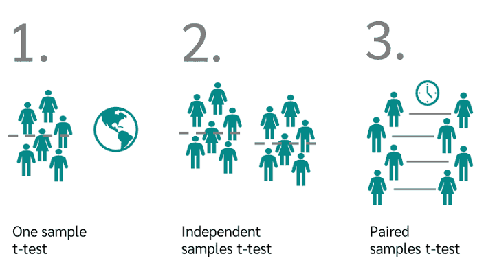
For example: in an attempt to measure the impact of micro-finance loans on poverty, a micro-finance institute has collected data on households who received loans and those who did not. Data was collected using the poverty probability index (PPI) methodology. An independent samples t-test would compare the PPI of the two groups. In a repeated measures t-test we could compare the PPI of the households who received a loan, at two points in time (e.g., one year and three years after the loan was granted) to measure short and long-term effects.
In this StatSnip we will show you how to use STATA and R, to apply the t-test to your data set.
The t-test is a special case of ANOVA (Analysis of Variance), for testing differences between two or more groups. ANOVA, in its turn, is a special case of regression analysis. That implies that, in principle, we might as well use regression analysis for testing differences!
For training your skills in interpreting output, we will use the dedicated commands for applying the t-test and the regression approach, in STATA and R.
We have randomly sampled from data on micro-finance (MF) applicants of a micro-finance institute (MFI). In order to assess the impact of MF loans, the MFI conducts a survey using the Poverty Probability Index (PPI) methodology. The charm of the PPI is that consists of 10 easy-to-answer questions which jointly predict the probability that a household is below or above the poverty line.
Not all applicants are granted a loan. The survey is conducted approximately one year after the MFI’s decision to accept or reject the application. Note that the decision to accept the application may be related to the income of the household at the time of the application, and hence the difference in PPI between successful and unsuccessful applicants is not necessarily caused by the loan!
Successful applicants are asked to participate in the survey biannually. We have limited our analysis to the first and second measurement. Obviously, repeated measurement data are not available for unsuccessful applicants.
In reality, the data on applicants is complex. Some of the unsuccessful applicants did have loans in the past, and/or have loans from other MFIs. The definition between successful and unsuccessful applicants is not clear-cut.
The data set contains four variables:
group and mf both refer to the status of the applicant. group = “NOMF” and mf=0 indicate that the respondent did not receive a loan. group = “MF” and mf=1 indicate that the application was successful.
ppi0 and ppi1 are the scores on the the PPI one and three years, respectively, after the decision on the application was taken. ppi1 is only available for successful applicants. The entries “NA” stand for Not Available.
You can browse through the data:
library(readstata13)
mf200 <- read.dta13("TTEST_DATA_01_sample200.dta")
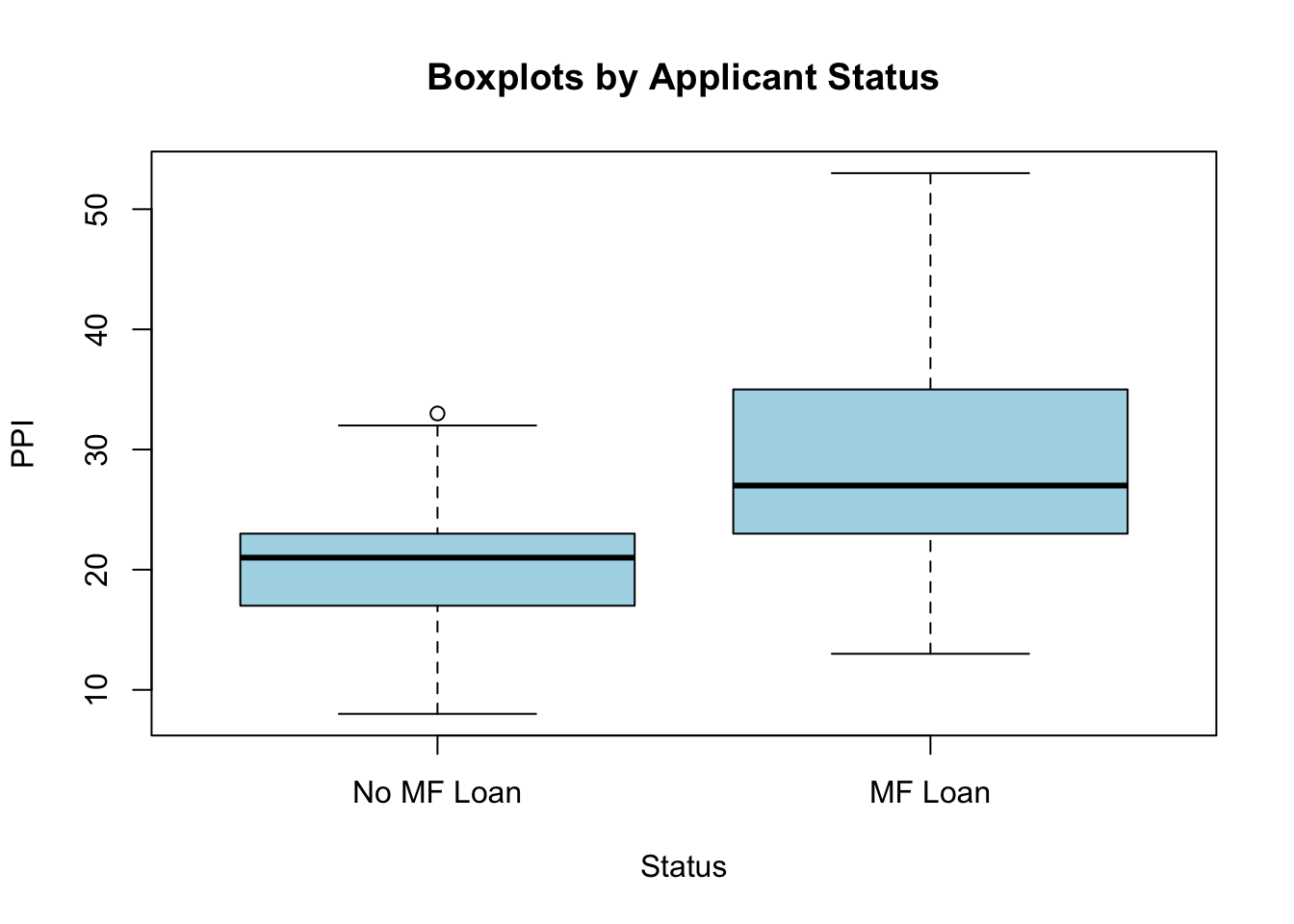
mf200It is always good to have an overview of the data before analysis. The best option here is to use a boxplot. A boxplot shows:
The median value, for each group.
The interquartile range.
Any outliers, or unusual values.
From the boxplot below we can conclude that:
All values of ppi0 are in the range of the scale (0 to 100).
The median of ppi0 is higher in the group of households with an MF-loan.
The minimum and maximum values of ppi0 are higher in the group of households who received an MF-loan.
# labels for Axis
label=c("No MF Loan","MF Loan")
# Boxplot
boxplot(ppi0~mf,
        names=label,
        data=mf200,
        main="Boxplots by Applicant Status",
        xlab="Status",
        ylab="PPI",
        col="Lightblue",
        border="Black"
)
A slight disadvantage of a boxplot is that it is hard to read the exact values of minimum, maximum, and median. Most of us would prefer to use the mean (or average) as a measure of central tendency, rather than the median.
There are many ways to get the descriptive statistics (often referred to as descriptives, after the command used in SPSS).
An easy way to get descriptives, is the describeBy() function in the psych package. A disadvantage is that it includes statistics that you do not need.
A more flexible alternative is the summaryBy() function from the doBy package. A disadvantage here is that you would need yet another package to get the skewness and kurtosis statistics - which are needed to assess the normality of the distribution. Also, the command is less compact than in the describeBy() option.
Below, we have used both options (but use Google to find more and even better options!).
We start with the summaryBy() option, and display the number of cases (respondents), the minimum, mean, median, and maximum values, the standard deviation, and the interquartile range of ppi0 for both groups. A cosmetic advantage is that the format of the output allows us to display the numbers in two decimals (or any other number you find convenient).
# install.packages("doBy")
library(doBy)
x <- summaryBy(ppi0 ~ mf, data = mf200,
          FUN = function(x) {
            c(n=length(x), min=min(x), mn = mean(x), md=median(x),
              max=max(x), sd = sd(x), iqr=IQR(x))
          } )
round(x,2)
We have refrained from adding the skewness and kurtosis. These are included in the describeBy() function.
library(psych)
describeBy(mf200$ppi0,mf200$mf)
 Descriptive statistics by group
group: 0
   vars  n  mean   sd median trimmed  mad min max range  skew kurtosis   se
X1    1 94 20.24 4.57     21   20.33 4.45   8  33    25 -0.08     0.26 0.47
------------------------------------------------------------
group: 1
   vars   n  mean   sd median trimmed mad min max range skew kurtosis   se
X1    1 106 29.03 9.48     27   28.49 8.9  13  53    40 0.51    -0.49 0.92
From the output we can read, for example, that the mean ppi0 (the PPI one year after the loan application), is 20.24 for households without an MF-loan, and 29.03 for households with an MF-loan. The skewness is 0.51, indicating that the distribution is slightly right skewed rather than symmetrical.
One assumption for a t-test is that the variable of interest is approximately normally distributed. If the assumptions for a t-test are violated, then it is better to switch to nonparametric tests. These will be discussed in a separate StatSnip.
In this section, we will apply the independent samples t-test and the paired sample t-test in STATA. We will also use regression analysis to achieve the same.
In the next section, we will do the same, using R.
In our data set we have data on PPI (one year after the decision on the loan application) for 200 respondents. 94 did not get the loan, and 106 did. We are interested in the difference in ppi0 between these two groups.
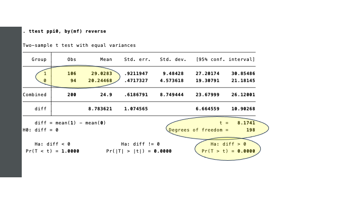
The vital information of the output of the STATA-command is marked yellow.
STATA’s ttest command is applied to the variable of interest (ppi0), for the two groups specified by mf (0 or 1, for households without and with an MF-loan, respectively). We have added the option reverse, since we assume that the mf=1 group has a higher ppi0. This is purely for ease of interpretation of the output, and does not affect the outcomes. By default, STATA would test the difference mean(0) - mean(1), and as a consequence the signs would change from plus to minus.
The test statistic (t) is computed as 8.17. The larger the difference between the means, the higher the value of t. The probably of t being as high as it is in our sample, under the null hypothesis that the means in the population from which the sample is drawn are equal, is close to zero.
In a one-sided test (with our alternative hypothesis ha < 0), the probability of t = 8.17, is p = 0.0000 (or zero).
It is common to use a 95% confidence level. That is, if p < 0.05 we reject the null hypothesis, and find support for our alternative hypothesis that the PPI of households with an MF loan is higher than for households without an MF loan.
The information in the table confirms what we already learned from the descriptive statistics: the mean PPIs in the two groups are 20.24 and 29.03. We can refer to this different as the effect size: the effect of having an MF loan is an increase in PPI of 8.78.
Note that the term effect size suggests a causal effect: the difference between the groups is caused by the MF loan. But this is not necessarily the case! For instance, maybe MF loans were allocated to households in a better position to repay the loan and the interest! Causality would run in the opposite direction!
Effect sizes are important! Above we concluded that the two groups have significantly different PPIs. Statistical significance is the result of two things: the magnitude of the difference (here 8.78), and the sample size. With very large sample sizes, even small differences (tiny effects) can be significantly different.
Is a PPI difference of 8.78 a small or a large effect? The answer to that question depends on the variance of PPI. In the boxplots we saw that the PPIs are in the range from 10 to 50, overall. The bulk of the values are in the range from slightly below 20 to around 35, and in that context a difference of 8.78 is substantial.
The interpretation of effect sizes is often subjective, and related to knowledge of the topic and experience. In our example, the difference can be considered large on statistical grounds, but if the effect is in fact much smaller than we are used to in different settings (countries; MFIs), the effect may be considered disappointingly small!
In order to have a more or less objective assessment of the effect size, various measures are used. For the t-test, a common measure of effect size is Cohen’s D. An alternative is the point bi-serial correlation coefficient β (pronounced beta, which is in fact a regression coefficient, as we will see). These and other measures can be easily obtained from STATA.
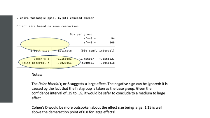
The table below provides a rough guide on the interpretation of effect size measures.
| Effect Size | Cohen’s D | β |
|---|---|---|
| Small | 0.2 | 0.10 - 0.30 |
| Medium | 0.5 | 0.30 - 0.50 |
| Large | 0.8 | >0.50 |
You are now ready to report the results of your analysis. When publishing your results in an academic thesis or a journal article, there are guidelines on how to report. Reporting the results of a t-test in APA-format, would give:
The mean test score for households with an MF loan was 29.03, with a standard deviation of 9.48. The mean test score for households without a loan was 20.24, with a standard deviation of 4.57. An independent samples t-test indicated that the t-statistic was 8.17, with df=198 (p < .05). The effect size is large (Cohen’s D = 1.16)
There is one thing that we have overlooked. In addition to the assumption of an (approximately) normally distributed variable in each group, the variances also have to be the same. Before applying the t-test, we have to test this. If the difference in variances is significant, then we can make a correction.
The sdtest command in STATA reveals that the variances are significantly different from one another, and therefore we repeat the ttest using the options unequal and welch. Unequal means that the variances are not equal, and Welch makes the correction the correction. You will note that the output is the same as without the correction, apart from the t-statistic and the degrees of freedom. The conclusion (a large and significant effect), remain the same.

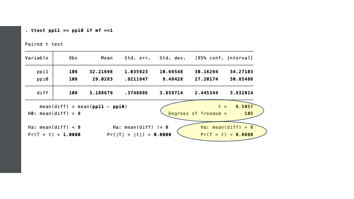
For the 106 households with an MF loan, we have two measurements: the PPI was measured one year (ppi0) and three years (ppi1) after the loan was granted. We now have a smaller group which is measured twice.
The test in STATA is straightforward.
Regression analysis is a popular statistical technique for modeling the relationship between a dependent variable, and one or more independent (or explanatory, or predictor) variables. For the sake of ease, we use the terms dependent and independent variables only.
Although the variables used in regression analysis are often numerical variables measured on ordinal, interval or ratio scales, in special cases we can use categorical variables for the dependent variable (e.g., logistic regression, in which the dependent variable is binary, 0/1-coded), and/or the independent variables. Binary, 0/1-coded, independent variables, are called dummy variables.
In our data set we have, for the independent samples t-test:
The general form of a regression model with one independent variable is:
\[ Y = \beta_0 + \beta_1 \times X_1 + \epsilon \]
The regression model for ppi0, predicted by mf:
\[ ppi0 = \beta_0 + \beta_1 \times mf + \epsilon \]
Since mf can only take on two values, 0 and 1, we can write for households without a loan:
\[ mf=0 \to ppi_{mf=0} = \beta_0 + \beta_1 \times 0 + \epsilon = \beta_0 + \epsilon \]
And for households with a loan:
\[ mf=1 \to ppi_{mf=1} = \beta_0 + \beta_1 \times 1 + \epsilon = (\beta_0 + \beta_1) + \epsilon \]
The coefficient β1 then represents the difference in the levels of ppi0 between the groups. Using a regression model, we can estimate β1 and test if it is significantly different from zero.
Referring to the video on t-test in the annex, the regression model then represents two horizontal lines, at levels β0 and β1.
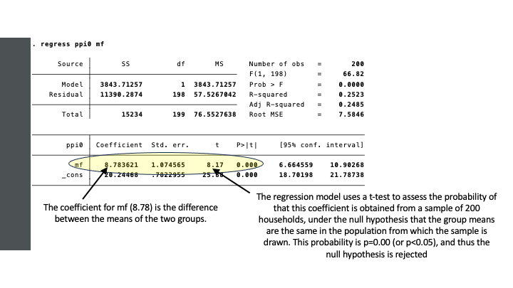
It is clear that the independent samples t-test and the regression approach, give the same results.
In the t-test, we addressed two issues:
1. Unequal group variances, necessitating a (Welch) correction.
2. Computation of the effect size (Cohen’s D, or a point-biserail correlation).
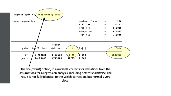
In STATA, we can use the robust option in regression and use the standardized regression coefficient, to obtain the same.
In summary:
| t-test | regression analysis | |
| Equal Group Variances | ttest t=8.1741; p=0.00 |
regress t=8.1741; p=0.00 |
| Unequal Group Variances | ttest, options unequal welch t=8.4870; p=0.00 |
regress, option vce(robust) t=8.4856; p=0.00 |
| Effect Size | esize, cohensd pbcorr Cohen’s D = 1.1581 r = 0.5024 |
regress, option beta - β (= r) = 0.5024 |
Regression analysis can also be used for paired samples. In our example, we ran a t-test to test the difference in PPI at two points in time, for the 106 households who received an MF loan. In essence, in the background, for each household the difference \(ppi1 - ppi0\) is computed. Next, it is tested whether the mean of differences is different from zero.
We can replicate the same using regression analysis. We first have to generate the differences (\(ppid = ppi1 - ppi0\)), and then use a regression model without independent variables. The constant (*_con*, in the output) then represents the mean difference, which is significantly different from zero. The values of t are identical, in both approaches.

It is a challenge to replicate and compare the outcomes of statistical methods across various software packages.
The charm of STATA is the integration of many statistical techniques in a systematic manner. In contrast, in R it is a bit harder to find your way.
Nevertheless, we do use R for several reasons. One reason is that it’s free. Another reason is that there are not many things that you cannot do in R!
For now, let’s see how we can obtain the same results as above, in R.
The t-test in R uses the t.test() function. Between the brackets, you specify the model, which uses the “~” (tilde) . The tilde means “(explained) by”. Here, **ppi0* is explained by the two groups.
# independent samples t-test
t.test(ppi0 ~ mf, mf200)
    Welch Two Sample t-test

data:  ppi0 by mf
t = -8.487, df = 155.24, p-value = 1.587e-14
alternative hypothesis: true difference in means between group 0 and group 1 is not equal to 0
95 percent confidence interval:
 -10.828033  -6.739209
sample estimates:
mean in group 0 mean in group 1
       20.24468        29.02830
Interestingly, by default, t.test() assumes that the group variances are not equal, and, hence the Welch-correction is applied. In general, it is considered good practice to assume equal variances unless a statistical test suggests otherwise! The order is: first test for equality of variances. If the test indicates that the variances are not equal, then you should use the Welch correction.
Below, we test for equality of variances. As we saw in STATA, the null hypothesis of equal variances is rejected, and therefore the default method is justified.
# test for equality of variances
var.test(ppi0 ~ mf, data = mf200)
    F test to compare two variances

data:  ppi0 by mf
F = 0.23255, num df = 93, denom df = 105, p-value = 7.615e-12
alternative hypothesis: true ratio of variances is not equal to 1
95 percent confidence interval:
 0.1567293 0.3467137
sample estimates:
ratio of variances
         0.2325472
If the variances are equal, then we have to specify it explicitly by the var-equal = TRUE option.
t.test(ppi0 ~ mf, mf200, var.equal=TRUE)
    Two Sample t-test

data:  ppi0 by mf
t = -8.1741, df = 198, p-value = 3.501e-14
alternative hypothesis: true difference in means between group 0 and group 1 is not equal to 0
95 percent confidence interval:
 -10.902683  -6.664559
sample estimates:
mean in group 0 mean in group 1
20.24468 29.02830 For the paired samples t-test, we use the same t.test() function, but the part between brackets looks different. We compare two variables, and there is no explanatory variable. That is, there is no tilde within the brackets.
# paired t-test
t.test(mf200$ppi1,mf200$ppi0,paired=TRUE)
    Paired t-test

data:  mf200$ppi1 and mf200$ppi0
t = 8.5057, df = 105, p-value = 1.345e-13
alternative hypothesis: true mean difference is not equal to 0
95 percent confidence interval:
 2.445344 3.932014
sample estimates:
mean difference
3.188679 The function for regression analysis is lm(), in R. lm stands for linear models.
The specification looks similar as in t.test(). Here, we store the results in an object labeled fit. A summary of that object gives detailed information.
fit <- lm(ppi0 ~ mf, data=mf200)
summary(fit)
Call:
lm(formula = ppi0 ~ mf, data = mf200)

Residuals:
     Min       1Q   Median       3Q      Max
-16.0283  -5.0283  -0.2447   3.7553  23.9717

Coefficients:
            Estimate Std. Error t value Pr(>|t|)
(Intercept)  20.2447     0.7823  25.879  < 2e-16 ***
mf            8.7836     1.0746   8.174  3.5e-14 ***
---
Signif. codes:  0 '***' 0.001 '**' 0.01 '*' 0.05 '.' 0.1 ' ' 1

Residual standard error: 7.585 on 198 degrees of freedom
Multiple R-squared:  0.2523,    Adjusted R-squared:  0.2485
F-statistic: 66.82 on 1 and 198 DF,  p-value: 3.501e-14
If the group variances are not equal, then we can use lm_robust, from the estimatr package. It is identical to lm().
# install.packages("estimatr")
library(estimatr)
fitrobust <- lm_robust(ppi0 ~ mf, data=mf200)
summary(fitrobust)
Call:
lm_robust(formula = ppi0 ~ mf, data = mf200)

Standard error type:  HC2

Coefficients:
            Estimate Std. Error t value   Pr(>|t|) CI Lower CI Upper  DF
(Intercept)   20.245     0.4717  42.916 3.139e-102   19.314    21.17 198
mf             8.784     1.0350   8.487  4.949e-15    6.743    10.82 198

Multiple R-squared:  0.2523 ,   Adjusted R-squared:  0.2485
F-statistic: 72.03 on 1 and 198 DF,  p-value: 4.949e-15
For the effect sizes, we can compute Cohen’s D and the point-biserial correlation.
The function for Cohen’s D is not part of base R. We can use a function in the lsr package.
When running this code on your computer, in R and RStudio, always remember to:
Install the package (via install.packages(“lsr”), in this case.
Invoke the functions in the package, via library(lsr).
The quotation marks are important!
# install.packages("lsr")
library(lsr)
#calculate Cohen's d
# Explanation:
# mf200[before comma,after comma] selects the rows (before comma) and columns (after comma)
# mf200[mf200$mf==0,3] selects all households without an MF loan (mf==0), and the third column in the data set (which is ppi0)
cohensD(mf200[mf200$mf==0,3], mf200[mf200$mf==1,3])
[1] 1.158081The point-biserial correlation can be obtained from the standardized regression coefficient, using the lm.beta() function from the package with the same name. Within brackets, you have to fill in the name of the object that contains the non-standardized results. We used fit.
# install.packages("lm.beta")
library(lm.beta)
lm.beta(fit)
Call:
lm(formula = ppi0 ~ mf, data = mf200)

Standardized Coefficients::
(Intercept)          mf
NA 0.5023061 For the paired samples t-test in R, we use the same strategy as in STATA. That is, we first compute a new variable ppid, which we then regress on a model with only a constant. The way to formulate that model is ppid ~ 1.
mf200$ppid <- mf200$ppi1 - mf200$ppi0
fitd <- lm(ppid ~ 1, data=mf200)
summary(fitd)
Call:
lm(formula = ppid ~ 1, data = mf200)

Residuals:
    Min      1Q  Median      3Q     Max
-6.1887 -3.9387  0.3113  2.8113  5.8113

Coefficients:
            Estimate Std. Error t value Pr(>|t|)
(Intercept)   3.1887     0.3749   8.506 1.34e-13 ***
---
Signif. codes:  0 '***' 0.001 '**' 0.01 '*' 0.05 '.' 0.1 ' ' 1

Residual standard error: 3.86 on 105 degrees of freedom
  (94 observations deleted due to missingness)
For paired samples, the effect size is computed as the mean of the difference divided by its standard deviation. You can do it, by computing the two components. Since we do have incomplete data (ppi1 is missing for households without an MF loan, and hence ppid can only be computed for households with an MF loan), we have to specify na.rm=TRUE (not available [missing] values, are removed).
mean(mf200$ppid) # generates NAs throughout[1] NAsd(mf200$ppid) # generates NAs throughout[1] NAdiffm <- mean(mf200$ppid,na.rm=TRUE) # missing values for ppid are ignored
diffsd <- sd(mf200$ppid,na.rm=TRUE) # missing values for ppid are ignored
# Effect size
effsize <- diffm / diffsd
cat("Effect Size is",round(effsize,4))Effect Size is 0.8261The table below summarizes what we have learned about implementing t-test in STATA and R.
For independent samples t-test we have:
| STATA t-test and regression | R t-test | R regression | |
|---|---|---|---|
| Equal Variances | t=8.1741 (df=198) | t.test(); var.equal=TRUE t=8.1741 (df=198) |
lm(y~x) t=8.1741 (df=198) |
| Unequal Variances | t=8.4870 (df=198) | t.test(y~x); default options t=8.4870 (df=198) |
lm.robust(y~x), from estimatr t=8.4870 (df=198) |
| Effect Size | Cohen’s D=1.1581 β = 0.5023 |
cohensd() from lsr 1.1581 |
lm.beta(model) β = 0.5023 |
For paired samples we have:
| STATA t-test and regression | R t-test | R regression | |
|---|---|---|---|
| Statistics | t=0.8507 (df=105) | t.test(y1,y2) t=0.8507 (df=105) |
lm(y~1) t=0.8507 (df=105) |
| Effect Size | mean/sd = 0.8261 | mean/sd = 0.8261 | mean/sd = 0.8261 |